Reusing datasets: from the abstract to the technical details
Overview
Teaching: 20 min
Exercises: 10 minQuestions
Which properties help us reuse datasets?
Objectives
Finding both data and software for reuse.
Visualising data from two different sets.
We want to find out, whether the Arctic and Antarctic ice core records show different temperature curves in the past. In order to do that, we can analyse ice core data from two different projects:
Please read both datasets’ abstracts now (North Greenland Ice Core Project Members 2007; Lorius et al. 1979).
- Noticed the DOIs & metadata? Both datasets are Findable.
- Noticed the
Downloadlinks overhttps? Easily accessible. - The list of parameters in both cases show that
Ageandd18O H2Owere measured. Looks interoperable. - CC-BY-licensed means we are allowed to reuse the material, if we “give appropriate credit, provide a link to the license, and indicate if changes were made.” :-)
However, will the data also be FAIR on the technical level, where we actually work? Will it be machine-reusable? We’re not going to use Excel for 8k datapoints, right?!
Let’s plan backwards from the the desired outcome: Comparing the temperature proxy measurements in a diagram. In order to get there, we need to:
- combine and/or align the x- and y-axes of both datasets,
- find out, whether we need to convert the values and/or units,
- extract the values from the dataset,
- know the datasets’ structures,
- download the datasets, and
- do all that in a reproducible manner ;-)
The last point makes it clear that we will work in a script file (.R
or .Rmd).
Challenge: How do we best download the datasets?
We could for example:
Download dataset as tab-delimited textmanually, save the files, then read them in.- Write our own little download function, e.g. with a vector of dataset IDs as input (
c(586886, 57629)).Which one do you prefer?
There is a third option ;-) Looking for an R package or a Python module related to the data repository. Search CRAN.R-project.org/web/packages/available_packages_by_name.html or ROpenSci.org/packages for “PANGAEA” (Chamberlain et al. 2018).
Challenge: Before installing your search result, check whether it seems useful.
How would you go about this in case of an R package or Python module?
Solution:
ROpenSci.GitHub.io/pangaear/reference gives an overview of its functions.
pg_data()sounds like what we need.
# install.packages("pangaear")
library(pangaear)
NGRIP <- pg_data(doi = "10.1594/PANGAEA.57629")
DomeC <- pg_data("10.1594/PANGAEA.586886")
Before analysing any data, we should get an overview of the R objects we created just now by the downloads:
str(NGRIP)
## List of 1
##  $ :List of 6
##   ..$ parent_doi: chr "10.1594/PANGAEA.57629"
##   ..$ doi       : chr "10.1594/PANGAEA.57629"
##   ..$ citation  : chr "Lorius, C; Merlivat, Liliane; Jouzel, Jean; Pourchet, M (1979): Isotope climatic record from ice core Dome C. P"| __truncated__
##   ..$ url       : chr "https://doi.org/10.1594/PANGAEA.57629"
##   ..$ path      : chr "/Users/katrinleinweber/Library/Caches/pangaear/10_1594_PANGAEA_57629.txt"
##   ..$ data      :Classes 'tbl_df', 'tbl' and 'data.frame':	434 obs. of  9 variables:
##   .. ..$ Depth ice/snow [m]     : num [1:434] 0.445 1.39 2.41 3.43 4.45 ...
##   .. ..$ Age [ka BP]            : num [1:434] 0.003 0.01 0.019 0.03 0.041 0.053 0.065 0.076 0.088 0.1 ...
##   .. ..$ Depth top [m]          : num [1:434] 0 0.89 1.89 2.93 3.93 4.97 5.97 6.86 7.77 8.67 ...
##   .. ..$ Depth bot [m]          : num [1:434] 0.89 1.89 2.93 3.93 4.97 5.97 6.86 7.77 8.67 9.47 ...
##   .. ..$ dD [per mil SMOW]      : num [1:434] -381 -388 -389 -389 -401 ...
##   .. ..$ d18O H2O [per mil SMOW]: num [1:434] -48.6 -49.6 -49.6 -49.7 -51.3 ...
##   .. ..$ d xs [per mil]         : num [1:434] 8.45 9.2 8.2 8.02 9.3 ...
##   .. ..$ Age min [ka]           : num [1:434] 0 0.006 0.014 0.024 0.035 0.047 0.059 0.07 0.082 0.094 ...
##   .. ..$ Age max [ka]           : num [1:434] 0.006 0.014 0.024 0.035 0.047 0.059 0.07 0.082 0.094 0.106 ...
##   ..- attr(*, "class")= chr "pangaea"
str(DomeC)
## List of 1
##  $ :List of 6
##   ..$ parent_doi: chr "10.1594/PANGAEA.586886"
##   ..$ doi       : chr "10.1594/PANGAEA.586886"
##   ..$ citation  : chr "North Greenland Ice Core Project Members (2007): 50 year means of oxygen isotope data from ice core NGRIP. PANG"| __truncated__
##   ..$ url       : chr "https://doi.org/10.1594/PANGAEA.586886"
##   ..$ path      : chr "/Users/katrinleinweber/Library/Caches/pangaear/10_1594_PANGAEA_586886.txt"
##   ..$ data      :Classes 'tbl_df', 'tbl' and 'data.frame':	4918 obs. of  2 variables:
##   .. ..$ Age [ka BP]            : num [1:4918] -0.05 0 0 0.05 0.05 0.1 0.1 0.15 0.15 0.2 ...
##   .. ..$ d18O H2O [per mil SMOW]: num [1:4918] -35.2 -35.2 -34.8 -34.8 -35 ...
##   ..- attr(*, "class")= chr "pangaea"
Both lists contain some metadata and the actual data as a tbl_df. What is that? Hint: It’s from the tidyverse.
In order to answer our research question (see above) we need to be able to combine
both the Age and the d18O.
To verify that both variables are really labelled in exactly the same way, we extract both tibbles and compare their variable names.
NGRIP <- NGRIP[[1]]$data
DomeC <- DomeC[[1]]$data
intersect(names(NGRIP), names(DomeC))
## [1] "Age [ka BP]" "d18O H2O [per mil SMOW]"
# less elegant, but also possible:
# c("Age [ka BP]", "d18O H2O [per mil SMOW]") %in% c(names(NGRIP), names(DomeC))
#> [1] TRUE TRUE
We get only exactly two variable names. This is great, because if there had been even the slightest difference in the name, unit, or a spelling mistake, we would have seen less output, because the names wouldn’t have intersect-ed.
We can now plot both datasets’ d18O H2O values against the same Age axis. Because the variables names contain spaces and brackets, we have to use the “back tick” character (`) around both. Snake_case colum names would have saved us from this, but hey!
library(ggplot2)
ggplot(data = NGRIP,
       mapping = aes(x = `Age [ka BP]`, y = `d18O H2O [per mil SMOW]`)) +
  geom_point(color = "dark green") + # inherits data & mapping from above
  geom_point(data = DomeC # overwrites above data, but inherits x & y
             ) +
  scale_x_reverse() # because Age means the past
## Warning: Removed 16 rows containing missing values (geom_point).
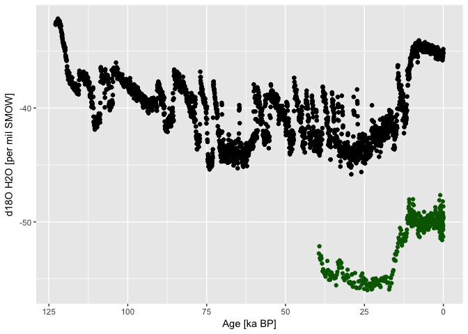
Incidentally, the Dome C core (black, east Antarctica) captured higher d18O
concentrations, than NGRIP (Greenland). Because of the inverse relationship
of d18O to temperature [@EPSTEIN1953213], it seems that the Southern Hemisphere
was been cooler than the North.
Conclusion
Integrating the two datasets with this little code was possible, because both variables are named exactly the same and thus easily machine-readable.
Granted, interoperability encompasses a few qualities besides uniform variable names. However, the datasets were well findable & accessible, and community-standard variable naming and the CC BY 3.0 license meant good reusability.
This is the power of FAIR Data combined with usable software: Reducing the burden of finding, downloading, cleaning up datasets, and actually using them.
Supplement: Harmonising different variable names
a) either rename one between downloading and plotting, or
names(NGRIP$`some other Age variable's name`) <- names(DomeC$Age_ka_BP)
names(NGRIP$`some other d18O variable's name`) <- names(DomeC$d18O_H2O_per_mil_SMOW)
b) specify in geom_point which second y should be plotted.
ggplot(data = DomeC,
       mapping = aes(x = `Age [ka BP]`, y = `d18O H2O [per mil SMOW]`)) +
  geom_point() +
  geom_point(data = NGRIP,
             mapping = aes(x = `some other Age variable's name`,
                           y = `some other d18O variable's name`)
             color = "dark green")
References
-
Chamberlain, Scott, Kara Woo, Andrew MacDonald, Naupaka Zimmerman, and Gavin Simpson. 2018. Pangaear: Client for the ’Pangaea’ Database. CRAN.R-project.org/package=pangaear.
-
Epstein, S, and T Mayeda. 1953. “Variation of O18 Content of Waters from Natural Sources.” Geochimica et Cosmochimica Acta 4 (5): 213–24. doi:10.1016/0016-7037(53)90051-9.
-
Lorius, C, Liliane Merlivat, Jean Jouzel, and M Pourchet. 1979. “Isotope climatic record from ice core Dome C.” Data set. PANGAEA. doi:10.1594/PANGAEA.57629.
-
North Greenland Ice Core Project Members. 2007. “50 year means of oxygen isotope data from ice core NGRIP.” Data set. PANGAEA. doi:10.1594/PANGAEA.586886.
Key Points
The FAIR-er a dataset, the easier its reuse in answering a new research question.